Market cycles. From a repeating pattern to a testable idea.

What is a market cycle?

A cycle is a recurring pattern in a measured series. A price cycle can be described by its period (bars between equivalent points), amplitude (size of the swing around its baseline), and phase (where in that swing the series is at a given time). One rise and fall alone gives too little evidence to establish recurrence.

• Statistical cycles are candidate rhythms estimated from data. They can move, fade or disappear as the sample changes.
• Calendar seasonality groups observations by a known schedule, such as calendar months. The calendar repeats even when the direction of returns varies.
• Economic cycles describe expansions and contractions in activity, credit or investment. Their duration varies, so an economic phase cannot be inferred from a price wave alone.

Different rhythms can overlap. A short wave can rise during a longer decline, and an observed price move also contains trend and irregular shocks. NBER business-cycle dating

Why do cycles form?

Repeated behaviour can come from scheduled activity, delayed responses or feedback. A retailer might build inventory ahead of a seasonal demand peak, then draw it down. An industry may expand capacity after strong demand, with the new supply arriving only after conditions have cooled. Changes in rates can affect borrowing, spending and investment through different channels and at different speeds.

These mechanisms are hypotheses to check against evidence. A peak in a spectrum cannot identify the cause of the pattern, and a few shocks or a changing trend can produce an apparent rhythm even without a stable cycle. Federal Reserve on monetary policy transmission

How to calculate a cycle

Example 1. Measure the spacing between peaks

Suppose three peaks in a synthetic daily series occur at bars 0, 25 and 50. The two peak-to-peak intervals are both 25 bars, so their average is 25 trading sessions. On a daily chart the count advances with trading observations. Check trough spacing and repeat the measurement in a later window before treating the estimate as stable.

Example 2. Fit a harmonic after removing the trend

Take log closes and subtract a linear trend estimated on the training window. For each candidate period T, regress the residuals on sine and cosine terms. Those two terms let the model estimate the wave’s phase without assuming where its peak falls.

For T = 25, a = 0.02 and b = 0, the fitted residual is +0.02 at bar 0, −0.02 halfway through the cycle at bar 12.5, and +0.02 at bar 25. Compare candidate fits on training data, then freeze the choice and score its errors on later bars against the trend-only baseline. For example, reducing a baseline error from 0.020 to 0.018 in the same error measure is a 10% relative improvement. That percentage measures model error. NIST spectral plot handbook

How cycles work in Delta Research

Statistical and Economic modes

Open Cycles → Configure cycles on the active daily chart. Statistical mode searches for local spectral peaks in linearly detrended log closes. The first 75% of the selected history identifies candidates with at least three training repetitions. The final 25% checks fixed-phase error against a training trend baseline. History presets and custom dates change the sample. Adaptive mode fits using a recent window based on 4, 6, 8 or 12 repetitions, with a floor of 120 observations.

Economic mode restricts the same search to editable reference bands. Defaults are Kitchin 2–5 years, Juglar 7–11, Kuznets 15–25 and Kondratiev 40–60. Delta converts years using the instrument’s observed bars per year and chooses the strongest eligible training fit in each band. Bands without enough history can be unavailable. A match to a named band gives a period hypothesis to investigate.

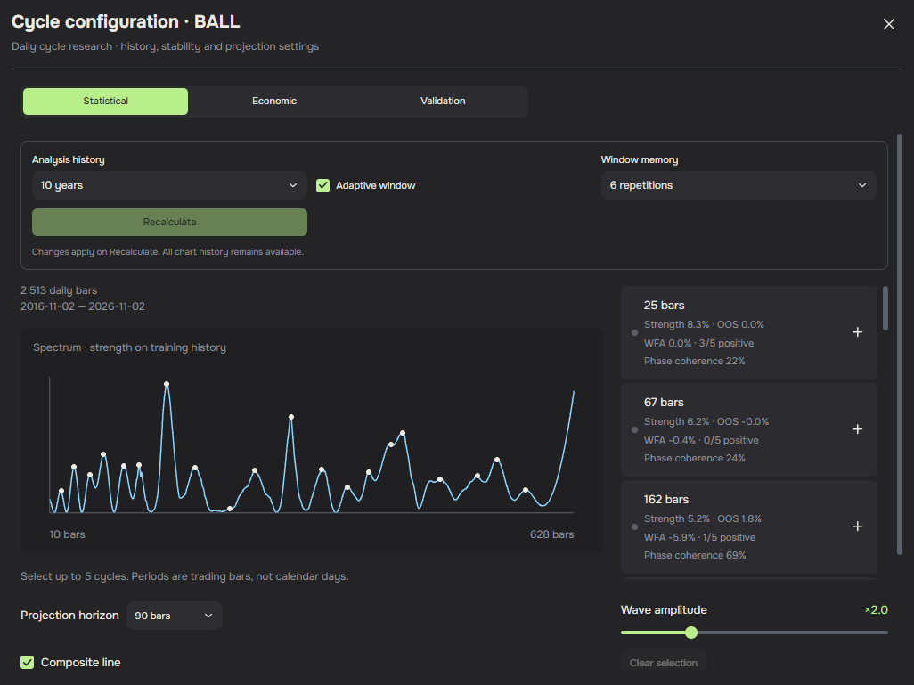
Read the validation before the projection

• Strength is the share of training residual energy explained by the candidate.
• OOS compares holdout error with the training trend baseline. A negative value means the model performed worse on that measure.
• WFA averages relative error improvement across eligible walk-forward folds. Each fold rediscovers and fits cycles using its own earlier data before testing the next segment. The positive-fold count tracks improved error, and matching today’s candidates to past discoveries makes this a retrospective diagnostic.
• Phase coherence measures how closely estimated phases line up across eligible folds. The validation view also reports stability and timing dispersion where available.

In the BALL snapshot, the 25-bar candidate has the highest displayed strength at 8.3%, but OOS and WFA round to 0.0%. The 162-bar candidate shows +1.8% OOS alongside −5.9% WFA and one positive fold out of five. The diagnostics give mixed evidence about whether the fitted rhythms carry forward.

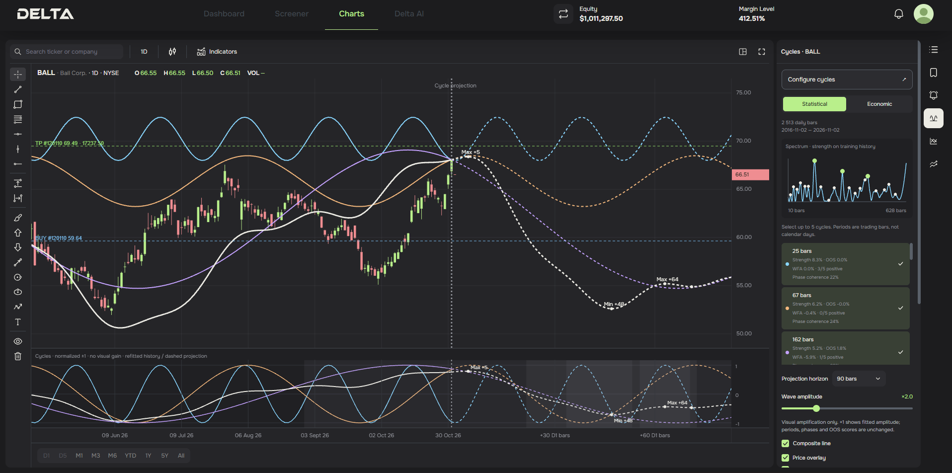
What the chart shows

Select up to five candidates. Coloured curves show individual waves. The white composite fits the selected periods jointly, with regularisation. Solid historical waves are refitted on the chosen sample. Dashed curves extend the model without extrapolating the trend. The price overlay is anchored to the last analysed close, while the lower pane shows normalised waves. The amplitude control changes the visual gain of the price overlay. Model scores, period, phase and the normalised pane stay the same.

The labels Max +5 and Min +48 in the example refer to extrema of the composite wave in trading bars from the analysis boundary. Any shaded timing spread summarises fold variation. It has no calibrated probability attached to it.

Use the cycle to define a watch window

Start with a candidate that shows evidence beyond its training fit. Specify a window around the projected turn and a separate condition based on observed prices. The window answers when to look. The condition tells you what evidence the setup requires.

In the synthetic example, a 25-bar harmonic with a five-bar phase advance projects a trough near bar 32.5. A hypothetical rule watches bars 31–33 for a low, then allows a confirmation through bar 35 if price closes back above a pre-marked level. The illustrated price line crosses that level at bar 34, so a close-based test can only evaluate the condition at that close and model execution on the next available bar. If price never confirms by bar 35, the example records no entry.

Before testing, define how the setup expires, what price action invalidates it, and how execution costs, liquidity and gaps affect the outcome. Recreate the analysis at each historical decision date using only data available then. Compare the same price rule with and without the cycle window on unseen periods, including transaction costs. This isolates whether the timing filter adds useful information.

Conclusion

A cycle model turns a visual impression into a measurable hypothesis. Estimate the period and phase, check whether they persist on later data, and require independent confirmation before counting a hypothetical entry. For the BALL snapshot, the mixed holdout and walk-forward results make it an example of how to read the tool and where to withhold confidence.